i. Integraph, Wikipedia, https://en.wikipedia.org/wiki/integraph gives a brief description with a couple of illustrations and a brief summary of its mechanism.

ii. Bruno Abakanowicz, Wikipedia, https://en.wikipedia.org/wiki/Bruno_Abakanoviwicz outlines his life and his many inventions

iii. Abdank-Abakanowicz Invents the Integraph, History of Information.com, http://www.historyofinformation.com/expanded.php?id=1565

iv. Polish Contributions to Computing, Bruno Abdank-Abakanowicz, http://chc69.fgcu.edu/EN/HistoryDetail/aspx?c=15 besides describing his integraph covers his other inventions. There is a good selection of references to his papers and other material.

v. Swiss Excellence: Gottlieb Coradi and his Instruments, Paoli Brenni, Bulletin of the Scientific Instrument Society No. 135, 2017

vi. Integrating with the Coradi Integraph Invented by Abdank Abakanowicz, Practical Technical Problems with Examples of Solutiions by Dr H Schilt published by G Coradi, Zurich, Switzerland. The first chapter can be downloaded from the Internet as a PDF file.

vii. Stanley, London, Stanley “A” Edition Catalogue (1958), author’s collection.

This paper was originally published in the Slide Rule Gazette, Issue 18, Autumn 2017 by the UK Slide Rule Circle.

Introduction

I have for many years wanted to add an integrator to my collection of mathematical instruments but the high prices asked by dealers, when one has occasionally appeared for sale, have always been more than I was willing to spend. Even offers through my web site email had come to nought, until now. However, on this occasion my website came up trumps and attracted the offer of this integraph, a deal was agreed, and it is now part of my collection (fig. 1).

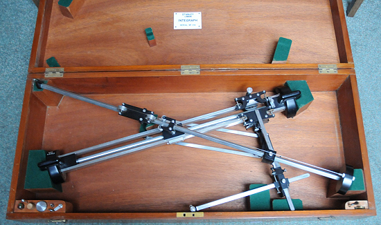
Figure 1

As can be seen it is quite different to the more common integrators that utilise polar planimeter technology. It is also a very large and heavy instrument. The case measures 90 x 41 x 19 cm and the instrument weighs 8.5 kg or 17.7 kg with its case. It is a metric scale version, catalogue no. A8606 in the 1958 Stanley catalogue, and was priced then at £332 - 15s (about half the annual salary of a draughtsman at that time). This Stanley example probably dates from the 1950s or 1960s and is serial no. 106. The digital computer would soon have made it redundant and this example has clearly seen little use; there is no sign of ink on the pen insert and the spare leads tube is full of unused leads. There was no lead in the pencil insert when I received it. Before launching into its construction and use it is, perhaps, worth saying a little about the history of this instrument.

History

There is quite a lot of information on the history and about its inventor on the Internet i,ii,iii,iv which I will summarise here. He was born in Ukmerge (Vilkmerge, Wilkomierz are alternative spellings), Lithuania (then part of the Russian Empire) on 6th October 1852. He is often referred to as being Polish as the town of his birth was at one time in the Polish-Lithuanian Commonwealth.

He graduated from Riga Technical University, Latvia and began an assistantship at Lwow Technical University. In 1881 he moved to France where he bought a villa in Parc St Maur on the outskirts of Paris.

In 1878 he developed the first working model of the integraph based on a principle introduced by Coriolis in 1836. And he patented his integraph in 1880. There then followed a period of development until 1889, the main difficulty being the transfer of direction to the knife edge wheel that creates the integral curve. His design of the integraph was taken up by the Swiss instrument maker Gottlieb Coradi  and the first version produced by his firm is illustrated in the Bulletin of the Scientific Instrument Society v as is also the later version introduced in the early 20th century. The Stanley Integraph is closely based on the second Coradi version.

Abakanowicz had several other patents including the parabolagraph, spirograph, the electric bell used in trains, and an electric arc lamp as well as publishing several works on a variety of mathematical and scientific subjects. He was an accomplished electrical engineer and his patents made him a wealthy man. He received the Legion d’Honneur in 1889. He died suddenly on 29th August 1900 (aged 47) in Saint-Maur-des-Fossés, France.

Description

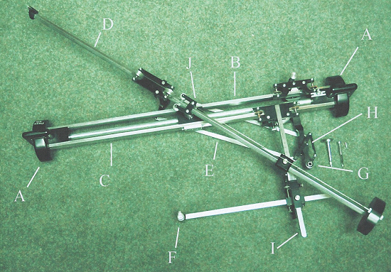
Figure 2

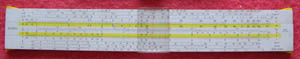
Fig. 2 shows the principle features of the integraph. The two wheels A, linked by an axle, carry the parallel beams B and C (which always remain parallel to the Y axis) and only allow movement in the direction of the X axis. Beam B carries a carriage connecting to the integrating wheel H and the pencil/pen holder G. Beam C carries a carriage connected to the guiding arm I to which is attached the tracing point F via another arm. A long rod D is mounted on the guiding arm I so that it can pivot. It also passes through a sliding and pivoting mount fixed to the centre of the two beams B and C. This rod carries a freely moving carriage below which is suspended one end of a parallel linkage E at the other end of which is the integrating wheel H. This wheel is sharp edged such that it will only move in a direction perpendicular to its axle, that direction being determined by the parallel linkage. Beam B carries a cm scale with a Vernier on its carriage. There is also a cm scale and micrometer adjusting screw on the guiding arm (base bar) for setting the position of the mounting position for the long rod D. This is used to set the desired base length,

Drawing the Integral Curve

With the fundamental curve mounted on the drawing board, the first requirement is to accurately position the instrument. To do this it must first be set to the orthogonal state (i.e. with the long rod D set at right angles to the two beams B and C). Once rotated to this position the carriage on beam C can be locked by engaging the screw 0n its front face with the recess in the centre of the front face of beam C. The tracing pin is now constrained to move in the direction of the X axis only and the instrument is now moved such that the tracing pin will accurately follow the X axis (Y = 0) of the fundamental curve. Whilst the instrument is being positioned the integrating wheel is held clear of the board by a screw located at the rear of the carriage on beam B. The tracing arm can be moved laterally by loosening the clamp to the guiding arm to ease the setting up.

The starting position of the carriage on beam B is arbitrary and needs to be set such that the integral curve will plot on the paper fixed to the drawing board for it without contacting the ends of the beam. Since the carriage on beam B will move in the same lateral direction as the tracing pin, the starting position should be set towards the opposite end of the beam. Assuming a suitable position has been found and the scale reading noted, with the integrating wheel now free to contact the board/paper and the integraph still locked in the orthogonal state, if the instrument is now moved to follow the X axis of the fundamental curve, it will draw the X axis of the integral curve.

Next set the tracing pin to the starting point (initial X value) on the X axis of the fundamental curve, unscrew the orthogonal locking screw, and accurately trace the fundamental curve to its final X value. This will draw the integral curve. The Y ordinate difference can now be accurately read from the Vernier on beam B.

A Simple Test

A simple test for which the analytical solution is well known is the bending of a simply supported beam with a uniformly distributed load. The fundamental curve in this instance is a rectangle. Fig. 3 shows the integraph set up on the drawing board for this test.

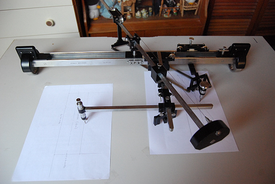
Figure 3

As expected the integral curve is an inclined straight line representing the shear force distribution. The fundamental curve can be written as f(x) = w where w (a constant) is the uniformly distributed weight and the integral curve ∫f(x) = wx. In fact the shear force diagram should run from wl/2 to
 -wl/2 (where l is the beam length) and the X axis needs to be moved in the Y direction by wl/2 to show the inverted diagram correctly and so that it can be used as the fundamental curve in order to produce the bending moment diagram. When used that way the expected parabola results. Fig.4 is a closer view of the first stage (drawing the shear force diagram).

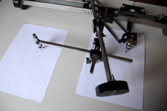
Figure 4

Appendix 1 – Fundamental Mathematical Principles

These were described in the first chapter of the book “Integrating with the Coradi Integraph”  vi and are repeated here.

a) The Indefinite Integral

Let y = g(x) be a function of which we wish to consider the indefinite integral

∫g(x) dx = ∫y dx

The integral is a new function, Y = G(x), which has the property that its differential quotient dY/dx is proportional to the function y = g(x) ; i.e.:  dY/dx = g(x)/λ

Here λ is a quantity independent of x ; it has the same dimensions as x and it is called the base of the integration. In mathematics the base is generally adopted as a unit of length and is therefore in most formulae not written at all. In what follows, however, it plays an important part.

Both the function y = g(x) and the function Y = G(x) can be represented by a curve; these are called the fundamental curve and integral curve respectively.

The indefinite integral and therefore the integral curve, is not completely determined by the definition given above, for every curve that is produced from Y by parallel movement in the direction of the Y axis possesses the property mentioned. The integral curve is only definitely determined when it is stated how great its ordinate is to be for x = x0.

b) Construction of the Integral Curve

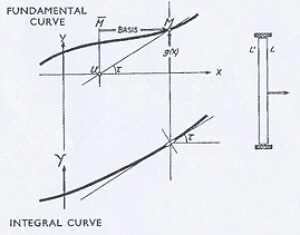
Figure 5

The integral curve can be constructed from its definition. From the point M in Fig. 5 the length λ (base length of the integration) MM is drawn to the left. The ordinate of M cuts the x axis at U. Then UM has the same direction as the tangent to the sought integral curve dY/dx = tan x.

If the problem is to br solved mechanically, we have only to move a pencil or a drawing board in the given direction UM. The problem can be solved, as Abdank-Abakanowicz perceived, with an integrating wheel. This is nothing else than a small, sharp edged, wheel which can move forward on the paper only in the direction of the plane of rotation (the plane normal to the axis of rotation). If the axis of the integrating wheel is always guided at right angles to the direction UM and moved forward uniformly with the ordinate of M, the integrating roller describes exactly the integral curve of the fundamental curve in question.

Appendix 2 – The Stanley ‘Allbrit’ Integrator Family

W F Stanley & Co Ltd are well known for their range of polar planimeters and derivatives such as radial planimeters, rule form planimeters and chart planimeters and many collectors will own one or more of these devices as polar planimeters, in particular, were made in tens of thousands. The planimeter itself is a simple form of integrator and its principle of operation could be extended by the use of suitable mechanisms to carry out higher order integration. W F Stanley produced a family of these integrators and related instruments of which the integraph was a member. The instruments in this family were very expensive, and more specialised, and hence were only made in much smaller quantities. They were described in the firm’s 1958 catalogue vii from where the images in this appendix have been taken.

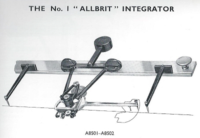The No. 1 is the simplest of these instruments. Like all the integrators it was made in inch and metric versions. It could determine the area, static moment and centre of gravity of plane figures, and volumes of solids of revolution. Looking at the figures you will see that is consists of a rail along which a counter-weighted carriage runs. The rail is aligned with the centre line of the figure to be traced using the projecting arms with pins at their ends. The figure was then traced in a similar manner to that used with a planimeter. At the forward end of the carriage the planimeter like, integrating wheel and graduated cylinder & disc can be seen On the opposite side of the carriage is the mechanism for providing the first (static) moment of area. In 1958 it cost £189 – 4s  (£189.20p). A typical application would be determination of  the stability of ship’s hull form (which depends on the vertical separation of the centre of gravity below the centre of buoyancy).

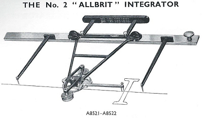
The No. 2 integrator has a second mechanism provided, similar to that for the static moment, for determining the second moment of area, commonly known as the moment of inertia. The application illustrated is the finding of the moment of inertia of the cross section of a beam. This is needed in order to determine the deflection of the beam and the resulting stresses under load. This model would typically have been used by civil and mechanical engineers. It cost £264 in 1958.

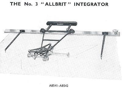The No. 3  integrator adds a third, similar mechanism for determining the third moment, which was of use in ballistic calculations. It cost £414 – 14s  (£414.70p), considerably more than the integraph that could also perform all these functions.

Often when these integrators appear on the market the beam, that had a separate case, is missing.

The harmonic analyser, shown in the last illustration is not actually used as an integrator but it also uses integrating technology in the form of polar planimeter arms that perform the calculation.

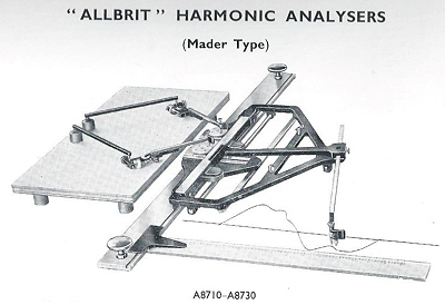By tracing the curve the instrument determines the harmonics that make up the complex waveform. The planimeters measure the areas enclosed by the paths traced out by two small depressions on the surface of gear wheels, the areas measured being proportional to the coefficients in a Fourier series representing the curve traced. A series of gear wheels was provided, one for each harmonic starting with the fundamental.

Three models were produced, No.1 (having only one planimeter) for determining the first six harmonics, one coefficient at a time, No. 2 with two planimeters and two sets of gears (as illustrated) for determining the coefficients two at a time, and No.3 for evaluation of harmonics 1 – 18. They were priced at £330, £357 -10s, and £407 respectively.

Figure 6

Figure 7

Figure 8

Figure 9